Diwanshu Jain, Roll No.: 150102016, Branch: ECE
Harshit Rajgadia, Roll No.: 150102024, Branch: ECE
Deepanshu Ajmera, Roll No.: 150102081, Branch: ECE
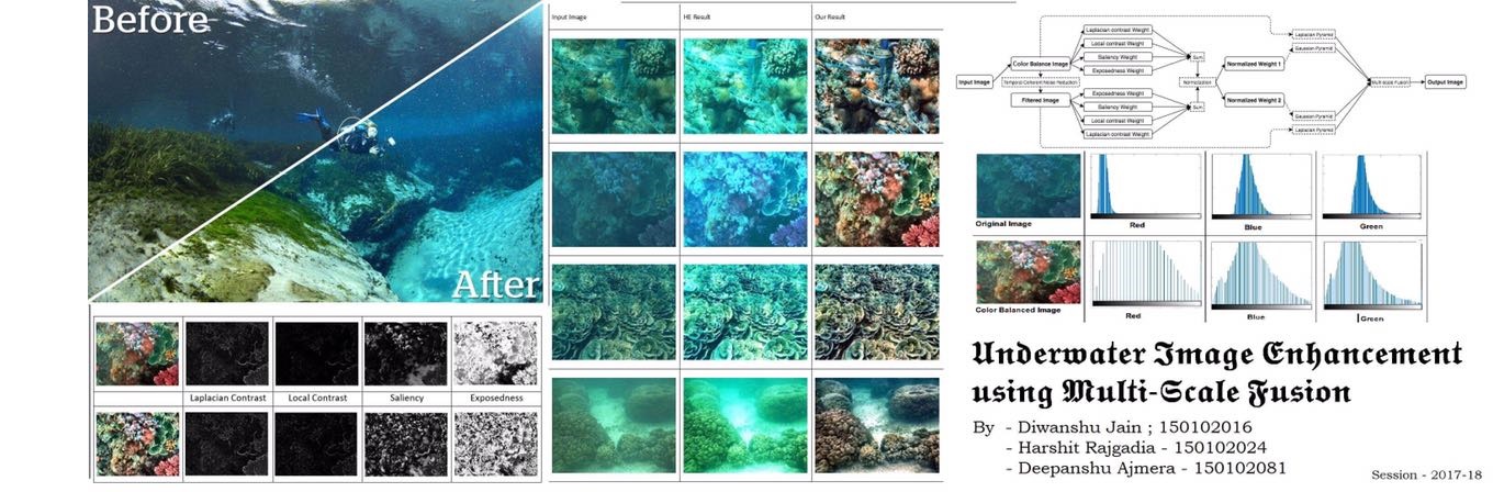
A novel approach is introduced that is able to enhance underwater images based on a single image. This approach is built on the fusion principle. In contrast to other methods, this fusion-based approach does not require multiple images, deriving the inputs and the weights only from the original degraded image. Since the degradation process of underwater scenes is both multiplicative and additive traditional enhancing techniques like color balance, color correction, histogram equalization shown strong limitations for such a task. Instead of directly filtering the input image, we used a fusion-based scheme driven by the intrinsic properties of the original image (these properties are represented by the weight maps). The success of the fusion techniques is highly dependent on the choice of the inputs and the weights and therefore we investigate a set of operators in order to overcome limitations specific to underwater environments. As a result, in our framework the degraded image is firstly white balanced in order to remove the color casts while producing a natural appearance of the sub-sea images. This partially restored version is then further enhanced by suppressing some of the undesired noise. The second input is derived from this filtered version in order to render the details in the entire intensity range.This fusion based enhancement process is driven by several weight maps. The weight maps of our algorithm assess several image qualities that specify the spatial pixel relationships. These weights assign higher values to pixels to properly depict the desired image qualities. Finally, this process is designed in a multi-resolution fashion that is robust to artifacts. Different than most of the existing techniques.
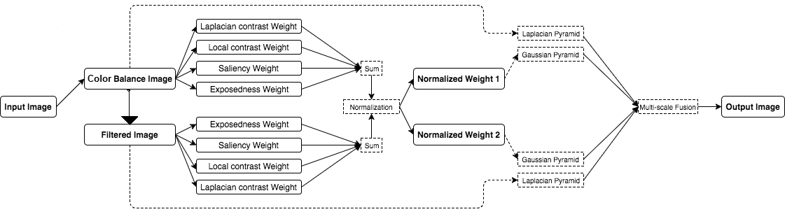
Figure 1: Functional Block Diagram
Zhang et al. introduced the haze optimized transformation (HOT), using the blue and red bands for haze detection, that have been shown to be more sensitive to such effects. Moro and Halounova generalized the dark object subtraction approach for highly spatially-variable haze conditions. A second category of methods, employs multiples images or supplemental equipment. In practice, these techniques use several input images taken in different conditions. Their main drawback is due to their acquisition step that in many cases is time consuming and hard to carry out.
We have implemented following paper for this project- "Enhancing Underwater Images and Videos by Fusion" -- Cosmin Ancuti, Codruta Orniana Ancuti, Tom Haber and Philippe Bekaert Hasselt University - tUL -IBBT, EDM, Belgium. Published in: Computer Vision and Pattern Recognition (CVPR), 2012 IEEE Conference on 26 July 2012. The link to the page can be found - here.
In short, Our enhancing strategy consists of three main steps: inputs assignment (derivation of the inputs from the original underwater image), defining weight measures and multiscale fusion of the inputs and weight measures.
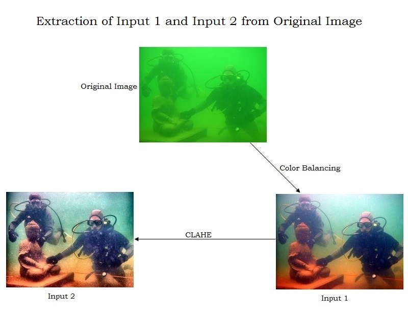
This enhancing solution does not search to derive the inputs based on the physical model of the scene, since the existing models are quite complex to be tackled. The first derived input is represented by the color corrected version of the image while the second is computed as a contrast enhanced version of the underwater image after a noise reduction operation is performed.
Under- and over-contrast occur in an underwater image whereas the amount of pixels is cumulatively concentrated at low and high intensity levels. Hence, stretching and clip-limit processes are applied to the image histogram of respective regions to prevent under- and over-contrast effects. We employed Simplest Color Balance method to implement this.
The idea is that in a well balanced photo, the brightest color should be white and the darkest black. Thus, we can remove the color cast from an image by scaling the histograms of each of the R, G, and B channels so that they span the complete 0-255 scale. In contrast to the other color balancing algorithms, this method does not separate the estimation and adaptation steps.In order to deal with outliers, Simplest Color Balance saturates a certain percentage of the image's bright pixels to white and dark pixels to black. The saturation level is an adjustable parameter that affects the quality of the output. Values around 0.01 are typical. Figure 2 shows the histogram of different channels after this step. Observe that the histograms has been stretched.
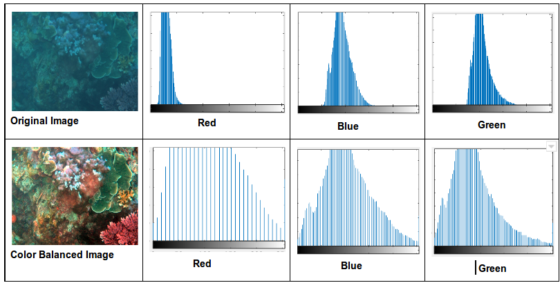
Figure 2: Histogram (input and output) in each channel after this step
In the fusion framework, the second input is computed from the noise-free and color corrected version of the original image. This input is designed in order to reduce the degradation due to volume scattering. To achieve an optimal contrast level of the image, the second input is obtained by applying the classical contrast local adaptive histogram equalization. To generate the second derived image common global operators can be applied as well. Since these are defined as some parametric curve, they need to be either specified by the user or to be estimated from the input image. Commonly, the improvements obtained by these operators in different regions are done at the expense of the remaining regions.The local adaptive histogram was opted since it works in a fully automated manner while the level of distortion is minor. This technique expands the contrast of the feature of interest in order to simultaneously occupy a larger portion of the intensity range than the initial image. The enhancement is obtained since the contrast between adjacent structures is maximally portrayed. To compute this input several more complex methods, such as the gradient domains or gamma correction multi-scale Retinex (MSR), may be used as well.
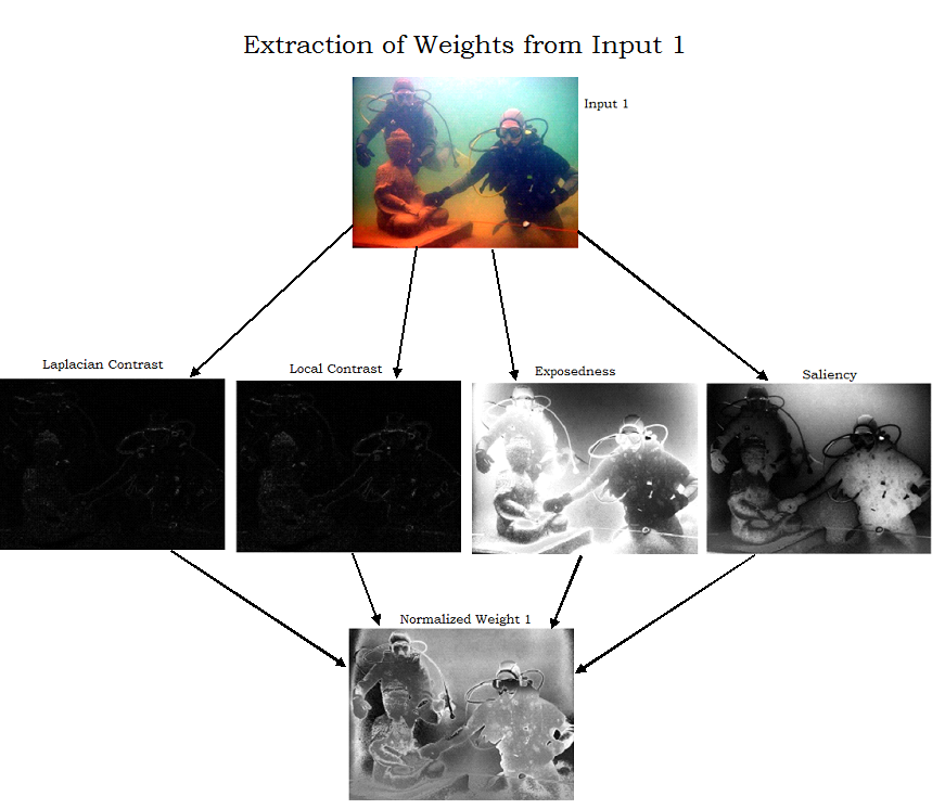
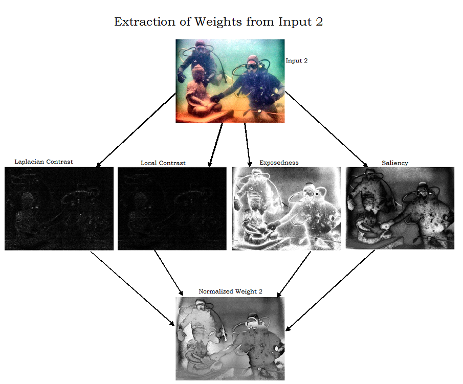
Laplacian contrast weight (WL ) deals with global contrast by applying a Laplacian filter on each input luminance channel and computing the absolute value of the filter result. This straightforward indicator was used in different applications such as tone mapping and extending depth of field since it assigns high values to edges and texture. For the underwater restoration task, however, this weight is not sufficient to recover the contrast, mainly because it can not distinguish between a ramp and flat regions. To handle this problem, an additional contrast measurement is used that independently assess the local distribution.
Local contrast weight (WLC ) comprises the relation between each pixel and its neighborhoods average. The impact of this measure is to strengthen the local contrast appearance since it advantages the transitions mainly in the highlighted and shadowed parts of the second input. The (WLC ) is computed as the standard deviation between pixel luminance level and the local average of its surrounding region:
WLC(x, y ) = ||Ik - Iωhck||
where Ik represents the luminance channel of the input and the Iωhck represents the low-passed version of it. The filtered version Iωhck is obtained by employing a small 5 X 5( (1/16)[1, 4, 6, 4, 1]) separable binomial kernel with the high frequency cut-off value ωhc = π/2.75. For small kernels the binomial kernel is a good approximation of its Gaussian counterpart, and it can be computed more effectively.
Saliency weight (WS ) aims to emphasize the discriminating objects that lose their prominence in the underwater scene. To measure this quality, the saliency algorithm of Achanta et al. was employed. This computationally efficient saliency algorithm is straightforward to be implemented being inspired by the biological concept of center-surround contrast. However, the saliency map tends to favor highlighted areas. To increase the accuracy of results, the exposedness map was introduced to protect the mid tones that might be altered in some specific cases.
Exposedness weight (WE ) evaluates how well a pixel is exposed. This assessed quality provides an estimator to preserve a constant appearance of the local contrast, that ideally is neither exaggerated nor understated. Commonly, the pixels tend to have a higher exposed appearance when their normalized values are close to the average value of 0.5. This weight map is expressed as a Gaussian-modeled distance to the average normalized range value (0.5):
WE(x, y) = exp((-(Ik(x, y) - 0.5)2)/(2σ2))
where Ik (x, y) represents the value of the pixel location (x, y) of the input image Ik , while the standard deviation is set to σ = 0.25. This map will assign higher values to those tones with a distance close to zero, while pixels that are characterized by larger distances, are associated with the over- and under- exposed regions. In consequence, this weight tempers the result of the saliency map and produces a well preserved appearance of the fused image.
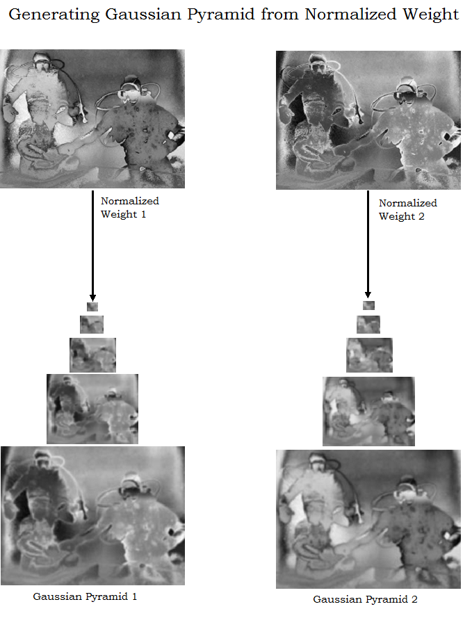
To yield consistent results, we employ the normalized weight values ϒ (for an input k the normalized weight is computed as ϒk = Wk /Σk=1K Wk ), by constraining that the sum at each pixel location of the weight maps W equals one.
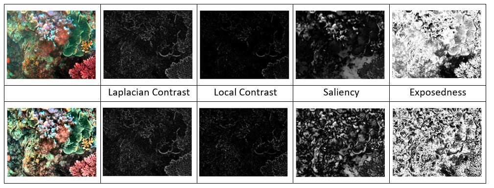
Figure 3: The two inputs derived from the original image and the corresponding normalized weight maps.
R(x, y)= Σk=1Kϒk(x, y) Ik(x, y)
where Ik symbolizes the input (k is the index of the inputs K = 2 in this case) that is weighted by the normalized weight maps ϒk. The normalized weights ϒ are obtained by normalizing over all k weight maps W in order that the value P of each pixel (x, y) to be constrained by unity value( ϒk = 1).
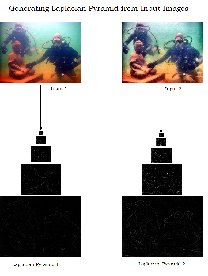
A common solution to overcome this limitation is to employ multi-scale linear or non-linear filters. The class of non-linear filters are more complex and has shown to add only insignificant improvement for this task . Since it is straightforward to implement and computationally efficient, in this experiments the classical multi-scale Laplacian pyramid decomposition has been embraced. In this linear decomposition, every input image is represented as a sum of patterns computed at different scales based on the Laplacian operator. The inputs are convolved by a Gaussian kernel, yielding a low pass filtered versions of the original. In order to control the cut-off frequency, the standard deviation is increased monotonically. To obtain the different levels of the pyramid, initially we need to compute the difference between the original image and the low pass filtered image. From there on, the process is iterated by computing the difference between two adjacent levels of the Gaussian pyramid. The resulting representation, the Laplacian pyramid, is a set of quasi-bandpass versions of the image.
In this case, each input is decomposed into a pyramid by applying the Laplacian operator to different scales. Similarly, for each normalized weight map ϒ a Gaussian pyramid is computed. Considering that both the Gaussian and Laplacian pyramids have the same number of levels, the mixing between the Laplacian inputs and Gaussian normalized weights is performed at each level independently yielding the fused pyramid:
Rl(x, y)= Σk=1KGl{ϒk(x, y)} Ll{Ik(x, y)}
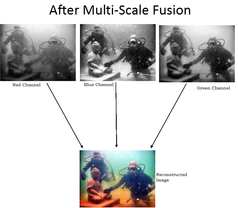
where l represents the number of the pyramid levels (typically the number of levels is 5), L{I} is the Laplacian version of the input I, and G W̄ represents the Gaussian version of the normalized weight map ϒ . This step is performed successively for each pyramid layer, in a bottom-up manner. The restored output is obtained by summing the fused contribution of all inputs.
The Laplacian multi-scale strategy performs relatively fast representing a good trade-off between speed and accuracy. By independently employing a fusion process at every scale level the potential artifacts due to the sharp transitions of the weight maps are minimized. Multi-scale fusion is motivated by the human visual system that is primarily sensitive to local contrast changes such as edges and corners.
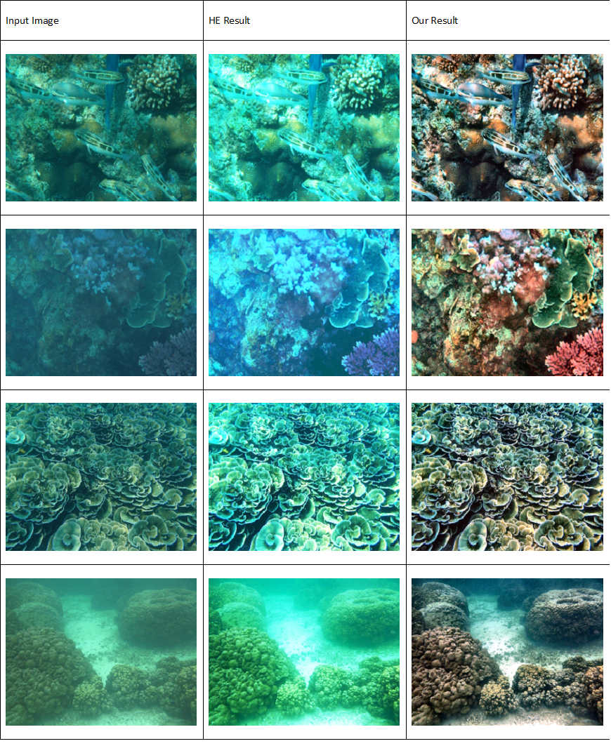
Figure 4: Comparision of outputs of MultiFusion technique and Histogram Equalization Method
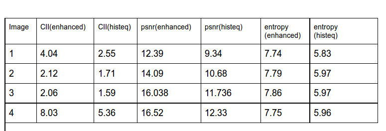
Figure 5: Quantitative analysis on several images using image quality index
nq= -log2N = -log2p
hi= -log2pi
H = Σipihi = -Σipilog2pi
AIC = Σk = 0L-1p(gk)log2(p(gk))
CII is the most important benchmark to compare the performance of various image enhancement techniques. It can be measured as a ratio of local contrast of final and input images. It can be represented by following equation-
CII = Aproposed/Aoriginal
We presented a fusion-based approach to restore underwater images. We demonstrate that by defining proper inputs and weights derived from the original degraded image they can be effectively blend in a multi-scale fashion to improve considerably the visibility range of the input underwater images.
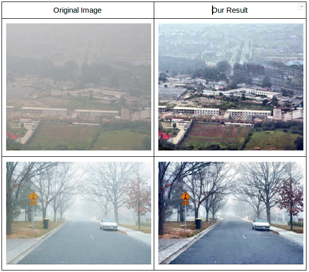
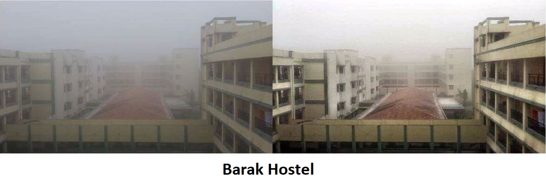
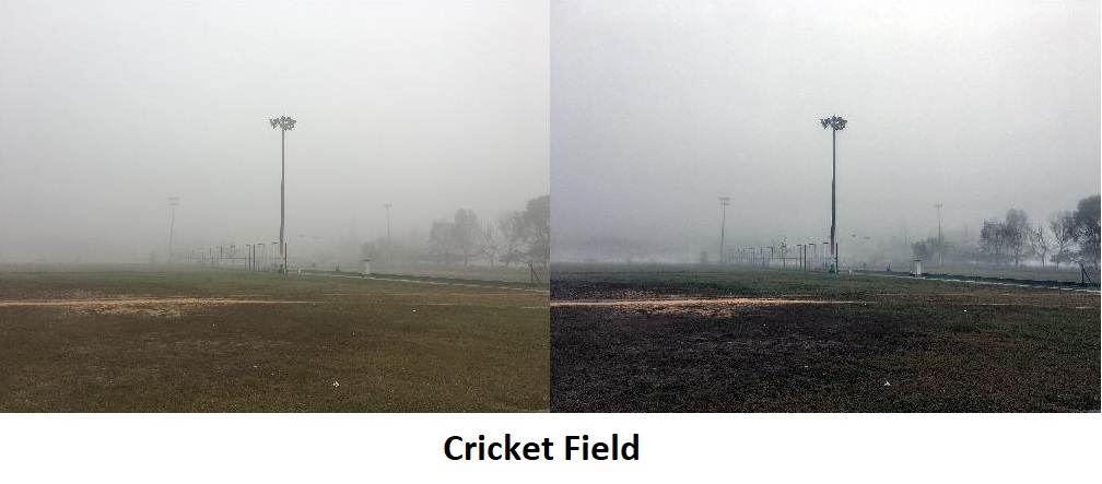
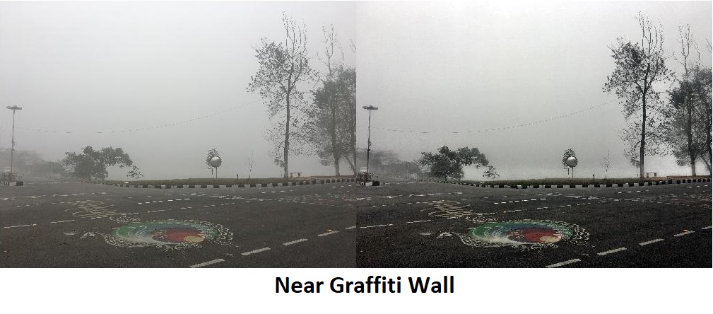
Figure 5: Our method on Atmospheric hazed images